Exploration of a lightcurve dataset with Self-Organizing Maps.
V. Belokurov (vasily at ast.cam.ac.uk), S. Feeney (smf35 at cam.ac.uk), W. Evans (nwe at ast.cam.ac.uk)
Modification history: ver. 2 | ver. 1
Self-Organizing Map (SOM) is a technique for monitoring and exploring large multi-dimensional datasets. A SOM is a list of reference vectors that span the data space in a way which is believed to preserve the local topology. The list is organized as a 2D grid of map nodes (neurons, processing units, whatever). Each datum is mapped onto a node associated with the nearest reference vector, e.g. the one with the smallest Euclidean distance from the data pattern. This distance is referred to as quantization error. To minimize the quantization error the winner node is shifted (in the data space) towards the corresponding datum and the neighbouring units (on the 2D grid) are alowed to share the adjustment. This concludes the description of the training algorithm. It can be seen that training a SOM can be done in no time even for large amounts of high dimensional data. For more information check out massive SOM bibliography.
SOMs are good because they train fast. Other advantages include:
unsupervised learning - good if you're out for coffee
natural clustering - no assumption is needed about the shape of clusters
novelty detection - large quantization error indicates that the input is either novel or rare
OGLE (Optical Gravitational Lensing Experiment) is a very succesful photometric survey. It is currently in its third phase. The second phase resulted in a catalogue of 220 000 variables objects in the direction of the galactic bulge. I band lightcurves from this catalogue were used to produce the SOM. More information on the OGLE's website.
To produce the SOM 50 000 random lightcurves were chosen from the catalogue. Power spectra were calculated (using Lomb-Scargle Periodogram), binned into 50 bins in a wide range of frequencies (periods from 1.1 day to 1000 days) and scaled to 1 at the maximum amplitude. For SOM training each 50-dimensional pattern was weighted according to the significance of the main peak in the spectrum.
SOM_PAK package was used to train the 50x30 map for 500 000 iterations with initial bubble size of 50 units. 500 000 iterations means each pattern was visited 10 times. This is normally considered as a short training phase during which some amount of large-scale ordering is achieved. Download SOM_PAK.
Once the map was trained the whole of 220 000 lightcurves were mapped onto it.
The figure below shows the distribution of distances between reference vectors. White corresponds to large distances; the distance decreases through violet, blue and green to yellow and red. Small distance means reference vectors look similar -- represent similar looking data patterns. One can define an object class as a group of nodes with a small relative distance surrounded by nodes with larger distance. For example a group of orange units at x=5, y=19 or a group of green units at x=46, y=5.
When you click on a node on the map the script returns a gzipped PostScript file with the lightcurves mapped onto this node. The PostScript page also contains the following information:
node coordinates
total number of hits for the node
mean quantization error for the patterns mapped on this node
For objects with period < 150 days lightcurves are wrapped around the period.
Each lightcurve panel contains the following information:
OGLE-II field number (1-49)
lightcurve number (starts from 0)
quantization error
period (if folded)
| Some examples. | ||
| Cataclysmic/Eruptive/Microlensing | ||
Node x=8, y=25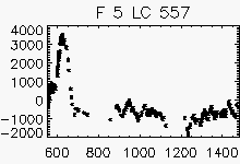
|
Node x=9, y=26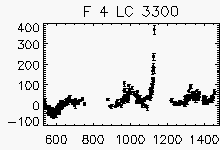
|
Node x=9, y=24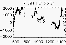
|
Node x=8, y=23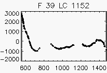
|
Node x=10, y=26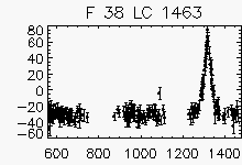
|
Node x=9, y=27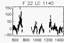
|
Node x=34, y=1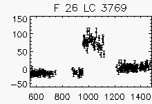
|
Node x=34, y=2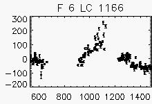
|
Node x=37, y=1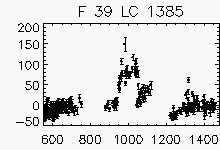
|
| Faulty lightcurves in the field 36 | ||
Node x=3, y=29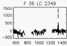
|
Node x=4, y=29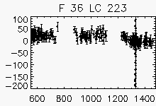
|
Node x=6, y=30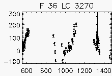
|
| Something very very long | ||
Node x=21, y=3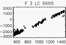
|
Node x=21, y=3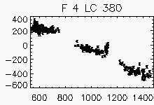
|
Node x=23, y=5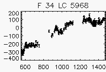
|
| Eclipsing binaries with period ~ 2 days | ||
Node x=46, y=2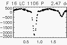
|
Node x=46, y=2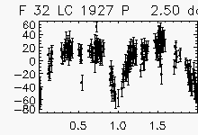
|
Node x=47, y=2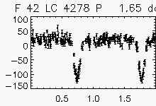
|
| Pulsating with period > 1 year | ||
Node x=2, y=2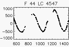
|
Node x=2, y=1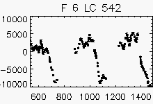
|
Node x=2, y=4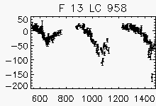
|