Exploration of a lightcurve dataset with Self-Organizing Maps.
V. Belokurov (vasily at ast.cam.ac.uk), S. Feeney (smf35 at cam.ac.uk), W. Evans (nwe at ast.cam.ac.uk)
Modification history: ver. 2 | ver. 1
Self-Organizing Map (SOM) is a technique for monitoring and exploring large multi-dimensional datasets. A SOM is a list of weight vectors that span the data space in a way which is believed to preserve the local topology. The list is organized as a 2D grid of map nodes (neurons, processing units, whatever). Each datum is mapped onto a node associated with the nearest weight vector, e.g. the one with the smallest Euclidean distance from the data pattern. This distance is referred to as quantization error. To minimize the quantization error the winner node is shifted (in the data space) toward the corresponding datum and the neighbouring units (on the 2D grid) are alowed to share the adjustment. This concludes the description of the training algorithm. It can be seen that training a SOM can be done in no time even for large amounts of high dimensional data. For more information check out massive SOM bibliography.
SOMs are good because they train fast. Other advantages include:
unsupervised learning - good if you're out for coffee
natural clustering - no assumption is needed about the shape of clusters
novelty detection - large quantization error indicates that the input is either novel or rare
OGLE (Optical Gravitational Lensing Experiment) is a very succesful photometric survey. It is currently in its third phase. The second phase resulted in a catalogue of 220 000 variables objects in the direction of the galactic bulge. I band DIA lightcurves from this catalogue were used to produce the SOM. More information on the OGLE's website.
We choose to construct the SOMs with high-quality lightcurves. So, the first job is to select these. This is done by allocating a rough measure of signal-to-noise ratio (S/N) to each lightcurve. The three maximum flux values and three minimum flux values are used to construct 9 flux differences Delta f. In each case, the noise is computed by adding the flux errors of the individual measurements in quadrature. This gives 9 estimates of S/N, of which of the minimum is selected to guard against outliers. The distribution of the S/N values is shown in this Figure. An empirically defined cut requiring the S/N to exceed 10 is imposed to select ~60,000 high-quality lightcurves.
Each of these is analysed with a Lomb-Scargle periodogram (Press et al. 1992). The power spectra are binned in the following way. First, we identify 5 ranges of interest (corresponding to the period intervals defined by the endpoints 1.11, 3, 9, 30, 100, 1000 in days). Each range is split into 10 equally-spaced bins in the frequency domain. The maximum value of the power spectrum in each bin is found. This gives a crude envelope for the shape of the power spectrum, which is now scaled so that its maximum value is unity. This associates each lightcurve with a 50-dimensional vector.
To this, 3 further pieces of information are added. The first is a magnitude difference Delta mag. From the distribution of flux measurements, the 2nd and 98th percentiles are found and converted to a flux difference in magnitudes using the zeropoint of the DIA analysis, given for each lightcurve by Wozniak et al. (2002). The second is the flux difference between the 98th percentile and the 50th (the median). This is normalised by the flux difference between the 98th and 2nd percentiles to give a number between zero and unity. This gives us a way of distinguishing between dips and bumps. Finally, the third is V-I colour. Each lightcurve has now been replaced by a 53 dimensional vector.
We are now ready to train the map. The map has 50 x 30 nodes, which gives a useful trade-off between resolution and speed. To initialise the map, we carry out a principal component analysis on the entire datacloud in the 53 dimensional space. The two most significant directions define a plane. Each weight vector is chosen to span this plane. To train the map we used SOM_PAK software (available for free download).
For the first phase, the initial size of the neighbourhood corresponds to the size of the map. The number of iterations is 5x10^5 and the learning rate is 10 per cent. The first phase establishes the large-scale ordering map. In the second phase, the initial size of the neighbourhood is 3, the number of iteration is 5x10^6 and the learning rate is 5 per cent. The second-phase fine-tunes the ordering on the map.
Once the map is trained the whole of 220 000 lightcurves are mapped onto it. The distribution of the quantization error is shown in this Figure.
When you click on a node on the map the script returns a gzipped PostScript file with the lightcurves mapped onto this node. The PostScript page also contains the following information: |
Each lightcurve panel contains the following information: For objects with period < 150 days lightcurves are wrapped around the period. |
To calibrate the map choose a
variable type from a drop-down menu below.
Shades of grey correspond to the number of hits of the chosen type of variability (white=large, black=small). Numbers inside nodes are the percentiles (from 1 to 100) of the node quantization error distribution cooresponding to the variable median error. Number less than 50 means the variable looks very similar to the majority of the lightcurves mapped onto a node and number close to 100 means it looks rather different. |
| ||
|
Contour | Variable stars |
|
|
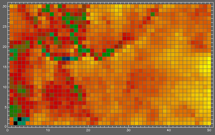
Umatrix shows the distribution of the distance between weight vectors | OSARG (8970 objects of type A and 6399 of type B) - OGLE Small Amplitude Red Giant variables in the Galactic Bar idetified by Wray, Eyer and Paczynski (data | paper) | |